Introduction to Vectors

1.1 Linear combination

Vectors

A vector is an object that has both a magnitude and a direction.

But for our purpose, consider vectors as groups of numbers.

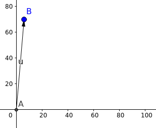
Let’s say I am 6ft tall and 70 kgs of weight, this information could be written as a vector.

\[\vec R = \begin{bmatrix}6\\70\end{bmatrix}\]

Graphically,

If I added my age to the vector then it would be plotted in a 3D space.

So, Vectors can be thought of as points in a n-dimensional space. These points are represented by a series of numbers which are the magnitudes of the vector to each axis of the n-dimensions.

Like, how 6 is my magnitude in the height axis and 70 is my magnitude in the weight axis.

Vector Operations

These Vectors can have some operations done on them.

Scalars

Let’s suppose a vector of house price and interest rate. And imagine if the prices and rates doubled. We would denote it as

\(\vec A = \begin{bmatrix}4\\5\end{bmatrix}, c = 2\) (4 crores, 5%)
\(c.\vec A = \begin{bmatrix}8\\10\end{bmatrix}\)

Here, $c$ is a scalar.
Scalars are numbers which scale a vector when multiplied with a vector. A scaled vector has the same direction or the opposite direction depending on whether it is scaled by a positive or negative scalar.

Addition

\[\vec C = \begin{bmatrix}0.5\\2\end{bmatrix}\] \[\vec R + \vec C = \begin{bmatrix}6+0.5\\70+2\end{bmatrix}\] \[\vec R + \vec C = \begin{bmatrix}6.5\\72\end{bmatrix}\]

It is like putting one vector at tip of another and seeing where it lands.

To add 2 vectors, you add the corresponding components.

For instance, let us suppose a Robot is as the origin in a 2D space. If we need to command it to go 5 meters forward in positive X-direction, and 3 meters forward in forward Y-direction, this command can be realized as a vector adiition as follows:
Initial position: I = (0,0)
Command: C = (5,3)
Final position: F = I + C

\(\vec I = \begin{bmatrix}0\\0\end{bmatrix}\)
\(\vec C = \begin{bmatrix}5\\3\end{bmatrix}\)
\(\vec F = \vec I + \vec C\)
i.e., \(\vec F = \begin{bmatrix}0\\0\end{bmatrix} + \begin{bmatrix}5\\3\end{bmatrix}\) i.e., \(\vec F = \begin{bmatrix}5\\3\end{bmatrix}\)

Subtraction

Subtracting 2 Vectors is just adding one vector and the negative of the other vector.
The negative of a vector is a vector with the same magnitude but opposite direction.

\[\vec R - \vec C = \begin{bmatrix}6-0.5\\70-2\end{bmatrix}\]

So, a vector subtraction can be understood as a combination of vector addition and a scalar multiplication
\(\vec A - \vec B = \vec A + (-1). \vec B\)

Linear Combination

In mathematics, a linear combination is an expression constructed from a set of terms by multiplying each term by a constant and adding the results.
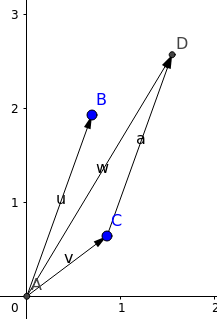
In the case of vectors Let $\vec A$ and $\vec B$ be 2 vectors and $c$ and $d$ be 2 scalars.
Then the linear combination is given by

\[c \vec A + d \vec B\]

Now, the combination can map to any point on the x y plane.

Let’s suppose we have

\[\vec A = \begin{bmatrix}60\\70\end{bmatrix}\] \[\vec B = \begin{bmatrix}100\\200\end{bmatrix}\]

and using this we want to map to

\[\vec Z = \begin{bmatrix}70\\80\end{bmatrix}\]

Then with $c = 1.68$ and $d = -0.44$ we can map to our point.

\[c \vec A + d \vec B\]

Like, this we can choose $c$ and $d$ such that we can map to any point in the xy plane.

Linear Combination of 3D Vectors

$\vec V$, $\vec W$ and $\vec U$ are 3 vectors in 3 dimensions.

$c,d,e$ are 3 scalars

The linear combination is

\[c\vec V + d\vec W+ e\vec U\]

Similar to 2D in 3D, combination of 2 vectors can map to any point on a plane. But this time it is not just the xy plane. This can be any plane.

A combination of of 3 vectors can map to any point in the 3D space.
But, if the third vector also lies on the plane that the combination of the first two vectors fill then it is not possible to fill the space. This is known as linear dependence then the third vector is said to be linearly dependent.

1.2 Lengths and Dot products

Dot product

\[\vec V.\vec W = V1*W1+V2*W2+V3*W3…\]

Length of a vector

To find the length of a vector first we need to calculate the Euclidean distance of the point from the origin.

\[Length ||V|| = \sqrt{(v1.v1+v2.v2+v3.v3...)}\] \[Length ||V|| = \sqrt{\vec V. \vec V}\] \[\vec V.\vec V = ||V||^2\] \[Length ||V|| = \sqrt{||V||^2}\]

Unit vector

A unit vector is a vector whose length is $1$. Example can be:

\[V = \begin{bmatrix}1/\sqrt{2} \\ 1/ \sqrt{2}\end{bmatrix}\] \[\vec V.\vec V = ½+½ = 1\] \[||V|| = \sqrt{1} =1\]

Basis vectors

A subset $B$ of vectors is called basis, if its elements are not linearly dependent, and every vector in the space is a linear combination of elements of B.

\[i = \begin{bmatrix}1\\0\end{bmatrix}\] \[j = \begin{bmatrix}0\\1\end{bmatrix}\] \[\vec V = \begin{bmatrix}49\\50\end{bmatrix}\] \[\vec V = 49\begin{bmatrix}1\\0\end{bmatrix} + 50\begin{bmatrix}0\\1\end{bmatrix}\] \[\vec V = 49i + 50j\]

Thus any vector can be represented as a linear combination of $i$ and $j$. So, $i$ and $j$ can be our basis for $R^2$.

If $\vec V$ is divided by its length/magnitude then the result is a unit vector in the same direction.

A unit vector $\vec U$ can also be denoted as

\[\vec U = \begin{bmatrix}cos\theta\\sin\theta\end{bmatrix}\]

Where $\theta$ is the angle made by the vector with $i$.
Any other vector $\vec V$ with length/magnitude $r$.

\[\vec V = \begin{bmatrix}r*cos\theta\\r*sin\theta\end{bmatrix}\]

Angles between vectors

The dot product is $\vec V$·$\vec W$ = 0 when $\vec V$ is perpendicular to $\vec W$.

The dot product of any vector with a zero vector is a zero vector. Hence zero vector is perpendicular to every other vector.

Cosine formula:

The cosine formula gives a measure of similarity (cosine similarity) given by the cosine of the angle between 2 vectors.

Let, $\vec A$ make an angle $\alpha$ with the x-axis

Let, $\vec B$ make an angle $\beta$ with the x-axis

\[\vec A = \begin{bmatrix}||A||cos\alpha\\||A||sin\alpha\end{bmatrix}\] \[\vec B = \begin{bmatrix}||B||cos\beta\\||B||sin\beta\end{bmatrix}\]

The unit vector in the direction of $\vec A$,

\[\vec {ua} = \frac{1}{||A||}\vec A-(i)\] \[\vec {ua} = \begin{bmatrix}cos\alpha\\sin\alpha\end{bmatrix}-(ii)\]

The unit vector in the direction of $\vec B$,

\[\vec {ub} = \frac{1}{||B||}\vec B -(iii)\] \[\vec {ub} = \begin{bmatrix}cos\beta\\sin\beta\end{bmatrix} -(iv)\]

Then, angle $\theta$, between $\vec A$ and $\vec B$ is given by

\(\theta = \alpha - \beta\) Assuming, $\alpha > \beta $, Now, $cos$ on both sides

\[cos\theta = cos(\alpha - \beta)\] \[cos\theta = cos\alpha cos\beta + sin\alpha sin\beta\] \[cos\theta = \begin{bmatrix}cos\alpha\\sin\alpha\end{bmatrix}.\begin{bmatrix}cos\beta\\sin\beta\end{bmatrix}\]

From $eqns$ $(ii)$ and $(iv)$

\[cos\theta = \vec {ua} . \vec {ub}\]

From $eqns$ $(i)$ and $(iii)$

\[cos\theta = \frac{\vec A.\vec B }{||A||*||B||}\]

Which also gives another definition for dot product

\[\vec A.\vec B = ||A||*||B|| * cos\theta\]

Where $\theta$ is the angle between the vectors.

Note: $\alpha$ > $\beta$ is not a necessary condition because
\(cos(\alpha - \beta) = cos(\beta - \alpha)\)

1.3 Matrices

Matrices are 2 dimensional arrangements of number.
They can be viewed as a group of column vectors or row vectors.

Multiplying matrix and vectors

When multiplying a matrix with a vector, we can perform linear combinations of the vector components with the corresponding columns of the matrix.

\[\vec X = \begin{bmatrix}x1 \\ x2 \\ x3\end{bmatrix}\] \[A = \begin{bmatrix}a & b & c \\ d & e & f \\ g & h & i\end{bmatrix}\] \[A\vec X = x1.\begin{bmatrix}a \\ d \\ g \end{bmatrix} + x2.\begin{bmatrix}b \\ e\\ h \end{bmatrix} + x3.\begin{bmatrix}c \\ f \\ i\end{bmatrix}\]

This gives an important insight. Unless the columns of the matrices are linearly dependent, a matrix can transform a vector to any vector in the space.

Matrix-vector multiplication can also be the dot product of the vector with each row of the matrix.

\[A \vec X = \begin{bmatrix}a & b & c & .(x1,x2,x3) \\ d & e & f & .(x1,x2,x3)\\ g & h & i& .(x1,x2,x3)\end{bmatrix}\]

Inverse matrix

In linear algebra, an $n \times n$ square matrix $A$ is called invertible (also nonsingular or nondegenerate) if there exists an $n \times n$ square matrix $B$ such that

\[A.B = B.A = I\]

Where $I$ denotes the $n \times n$ identity matrix and the multiplication used is ordinary matrix multiplication. If this is the case, then the matrix $B$ is uniquely determined by $A$ and is called the inverse of $A$, denoted by $A^{-1}$.

Linear Dependence

Linear dependence, in a set of vectors, is when one vector can be produced by the linear combination of the any other vectors in the set.

In other words,
A set of vetors ${ \vec V_{1}, \vec V_{2},… , \vec V_{n} }$ are said to be linearly dependent if

\[c_{1} \vec V_{1} + c_{2} \vec V_{2}+... + c_{n} \vec V_{n} = 0\;(zero\;vector)\]

When $0$ $\notin$ $c= { c_{1},c_{2},… ,c_{n}}$

Singular Matrix

It is a square matrix that doesn’t have an inverse.

Consider a matrix, \(A = \begin{bmatrix}3&6\\1&2\end{bmatrix}\)

In terms of linear dependence, a singular matrix has linearly dependent columns vectors.

\[-2 \begin{bmatrix}3\\1\end{bmatrix} + \begin{bmatrix}6\\2\end{bmatrix}= \begin{bmatrix}0\\0\end{bmatrix}\]

Solving linear equations

Linear equations are equations that describe the characteristic of a straight element in an $N_d$ space.
Solving the linear equations of 2 lines gives their point of intersection.
Solving the linear equations of 3 planes in 3D space gives their point of intersection.

2.1 Vectors and linear equations

\[x-2y = 1\] \[3x + 2y = 11\]

With reference to Gilbert Strang’s book “Introduction to Linear Algebra”. In this chapter the author paints 2 pictures to to depict linear equations.

Row picture

The row picture shows two lines meeting at a single point. The solution for x and y comes by figuring out where these lines meet. This can be done by finding y in terms of x in one equation. then substituting the y in the other equation.

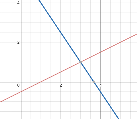
This picture is good for 2 or 3 dimensions but it becomes impossible to visualize in the higher dimensions.

Column picture

\[x\begin{bmatrix}1\\3\end{bmatrix} + y \begin{bmatrix}-2\\2\end{bmatrix} = \begin{bmatrix}1\\11\end{bmatrix}\]

Now in this picture a system of linear equations can be viewed as a linear combination of vectors.

My own preference is to combine column vectors. It is a lot easier to see a combination of four vectors in four-dimensional space, than to visualize how four hyperplanes might possibly meet at a point. (Even one hyperplane is hard enough. . . )

-Gilbert Strang

Matrix form of equations

A is a matrix of the coefficients of the equations. X is a vector of the variables of the equations.

\[A\vec X = B\] \[\begin{bmatrix}a & b & c \\ d & e & f \\ g & h & i\end{bmatrix}\begin{bmatrix}x \\ y \\ z\end{bmatrix} = \begin{bmatrix}b1 \\ b2 \\ b3\end{bmatrix}\]

2.2 Idea of Elimination

The aim of elimination is to get upper triangular form.
We subtract rows from other rows such that the such that some specific coefficients are 0.

What is a pivot?

It is the first non zero number in the row that does the elimination. In the example below, 4 is the pivot for row 1.

What is a multiplier?

The number to be eliminated, divided by the pivot, serves as the multiplier. In the example below, $\frac{3}{4}$ is the multiplier.

We multiply row 1 by the multiplier and subtract it from row 2 to get 0 in the position below the pivot.

But there can be situations when there are infinitely many or no solutions. We’ll call situations as failure conditions.

Failure conditions

There is no solution when the lines are parallel. If the lines never meet how can there be a point of intersection.

There are $\infty$ solutions if the lines are collinear.

We must remember that 0 can never be a pivot.

We need to exchange rows if a pivot is zero if such row is available.

The best situation is when n no of pivots exists for n equations.

Change to U matrix.

Use the first equation to make the first column all zeros under the first element.

\[\begin{bmatrix}1 & 1 & 0 \\ 1 & 2 & 1 & multiply\; row_1\; by\; (1/1)\; and\; subtract\\ 0 & 1 & 2 & multiply\; row_1\; by\; (0/1)\; and\; subtract\end{bmatrix}\] \[= \begin{bmatrix}1 & 1 & 0 \\ 0 & 1 & 1 \\ 0 & 1 & 2 \end{bmatrix}\]

Use the second equation to make the second column all zero under the second diagonal element.

\[= \begin{bmatrix}1 & 1 & 0 \\ 0 & 1 & 1 \\ 0 & 1 & 2 & multiply\; row_2\; by\; (1/1)\; and\; subtract\end{bmatrix}\]

\(= \begin{bmatrix}1 & 1 & 0 \\ 0 & 1 & 1 \\ 0 & 0 & 1 \end{bmatrix}\) And so on.

Summary

• Vectors can be thought of as points in a n-dimensional space. These points are represented by a series of numbers which are the magnitudes of the vector to each axis of the n-dimensions.

• The linear combination of 2 vectors is given by

\[c \vec A + d \vec B\]

• Dot product

\[\vec V.\vec W = V1*W1+V2*W2+V3*W3…\]

• Length of a vector

\[Length ||V|| = \sqrt{||V||^2}\]

• A unit vector is a vector whose length is $1$.

• Linear Dependence in a set of vectors, is when one vector can be produced by the linear combination of the any other vectors in the set.

• The matrix $B$ is the inverse of $A$ iff

\[A.B = B.A = I\]

• Linear equations can be solved by taking the equation to upper triangular form

• A is a matrix of the coefficients of the equations. X is a vector of the variables of the equations.

\[A\vec X = B\] \[\begin{bmatrix}a & b & c \\ d & e & f \\ g & h & i\end{bmatrix}\begin{bmatrix}x \\ y \\ z\end{bmatrix} = \begin{bmatrix}b1 \\ b2 \\ b3\end{bmatrix}\]

• Our aim is to change $A$ into $U$. Where $U$ is an upper tringular matrix.

Co-author: Anish Shrestha (https://www.linkedin.com/in/anish-shrestha-a99759144/)

References

1. Introduction to Linear Algebra, W. G. Strang
2. Gilbert Strang lectures on Linear Algebra (MIT), W. G. Srtang (https://www.youtube.com/watch?v=ZK3O402wf1c&list=PL49CF3715CB9EF31D&index=2)
3. Essence of linear algebra : https://www.3blue1brown.com/